Urban Resilience – Dar es Salaam
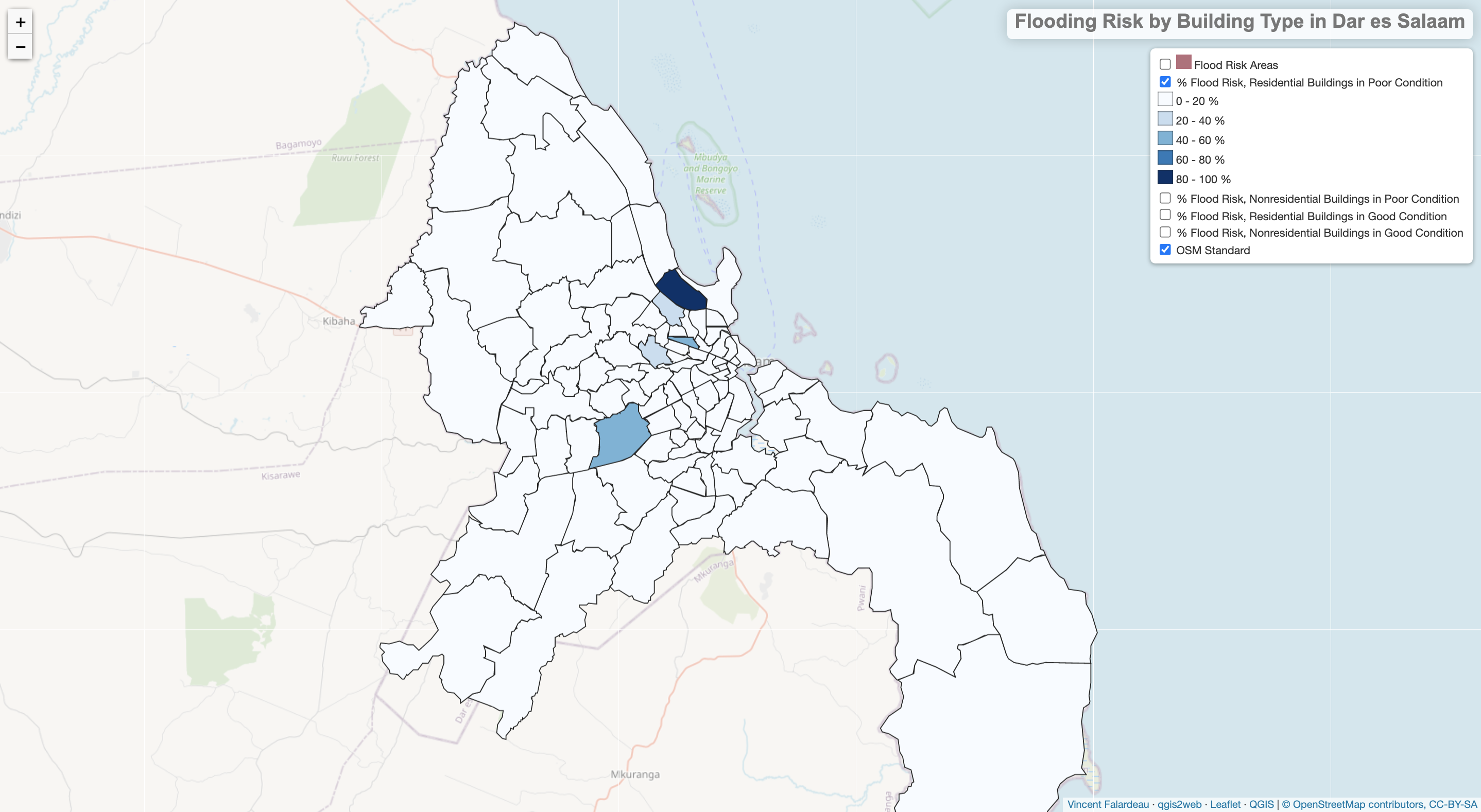
LEAFLET MAP: Flooding Risk by Building Type in Dar es Salaam
Complete SQL code for the analysis: Flooding_BuildingTypes_DarEsSalaam.sql
Questions
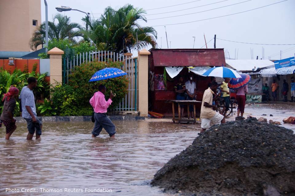
On the coast of the Indian Ocean, the city of Dar es Salaam is particularly susceptible to flooding. This analysis will investigate whether certain types of buildings are more likely to fall within areas that are vulnerable to flooding. Specifically, comparisons can be made between residential and nonresidential buildings, and buildings in poor vs. good condition. OpenStreetMap data for buildings in Dar es Salaam contains a “building” field that can be converted to a binary of residential/nonresidential, and for a smallish subset of buildings (approximately 80,000 of more than a million) there is also a sub-attribute, “building:condition” that specifies whether the structure is in a good or bad state. We can identify whether certain wards or neighborhoods in the city are at greater risk of flooding, and whether certain kinds of buildings are at the greatest risk within the high-risk wards. Generally speaking, residential buildings are of greater concern than nonresidential ones, and buildings in a poor condition might deserve more attention than ones in a good condition, since they could suffer more severe damage from floods. In the Methods and Code section to follow, I elaborate a procedure for calculating the ward-level percent risk for four categories of buildings – res/poor, nonres/poor, res/good, and nonres/good. It should be noted that in many wards there are no buildings with a specified “building:condition”, and these wards result in null values (in the leaflet map linked above, there is a blank space where the Pct Risk would be). (For this reason, I plan to expand this analysis to include all buildings in Dar es Salaam, calculating the percent risk for only two building categories, res and nonres. This will require a simple, modified repetition of the same steps that went into the four-category analysis, but it will take some time to make the necessary code changes.)
Data Sources
- OpenStreetMap data:
- Building polygons within Dar es Salaam. Three layers were used in this project: a set of all the buildings, including those without a “building:condition” specified; a file for all the buildings in poor condition; and one for all the buildings in good condition (obtained from the OSM API through the steps outlined below).
- Resilience Academy data:
- Administrative wards, as a Web Feature Services (WFS) layer, imported into PostGIS.
- Flood Scenario, 25-200cm, another WFS-format layer.
Much of OpenStreetMap’s data in Dar es Salaam consists of contributions from the Ramani Huria project. Ramani Huria is also closely involved with the Resilience Academy; both are initiatives of the Tanzania Urban Resilience Program (TURP), and Ramani Huria works towards training university students to collect geographic data in Dar es Salaam.
Methods and Code
To start, in the code editor side of https://overpass-turbo.eu, enter the following command to select buildings in Dar es Salaam classified as being in poor condition. Using this website allows you to query OpenStreetMap data, obtaining a smaller subset for download.
area[name="Dar es Salaam"];
nwr["building:condition"="poor"](area);
out center;
Then hit Run in the top left. If a popup window appears saying that the size of the data might pose an issue, click to continue anyway. When the process has finished running, click Export and navigate to Data – download as GeoJSON, which will create a file called export.geojson. Within the DB Manager for PostGIS, you can then click the icon labeled Import Layer/File, browse to the location of the file, and load it in to your database. For good measure, check the boxes for converting field names to lowercase and creating a spatial index. Repeat these query steps for buildings in good condition, starting from the Overpass Turbo selection:
area[name="Dar es Salaam"];
nwr["building:condition"="good"](area);
out center;
Now we have a layer consisting of the buildings that are in poor condition, and may therefore be especially vulnerable to flooding. As of April 6, 2021 there were 12,821 such buildings marked in Dar es Salaam. We also now have a layer of buildings in good condition, of which there are 69,402. I have renamed my export.geojson downloads to poorb.geojson and goodb.geojson, so subsequent queries will refer to poorb and goodb. We can run this query to get an idea for the types of building materials in poor buildings:
SELECT "building:material", count("building:material") as count_build_mat
from poorb
group by "building:material"
order by count_build_mat desc;
This yields the following result:
| building:material | count_build_mat |
|---|---|
| cement_block | 11629 |
| plaster | 349 |
| metal | 253 |
| wood | 176 |
| brick | 130 |
| waste_material | 38 |
| stone | 20 |
| concrete | 19 |
| glass | 4 |
| earthen | 3 |
| wood and steel binder | 1 |
| Steel | 1 |
It’s good to know, but might not be of much use to us, since almost all of the buildings are of cement block construction.
The next thing we want to do is to classify buildings as residential or nonresidential. First, we need to know what kinds of labels are assigned to buildings. Then we will be able to write a query that captures the full nuance of residential buildings.
-- Add an empty column “res_status” to the table to fill out with text entries, ’residential’ or ‘nonresidential’
ALTER TABLE poorb
ADD COLUMN res_status text;

-- Figure out what types of buildings there are, and how many of each kind:
SELECT "building", count("building") as count_build
from poorb
group by "building"
order by count_build desc;
This yields a table that shows most buildings in poor condition are residential:
| building | count_build |
|---|---|
| residential | 10556 |
| commercial | 882 |
| commercial;residential | 607 |
| construction | 335 |
| school | 141 |
| utility | 62 |
| public | 59 |
| yes | 54 |
| church | 39 |
| industrial | 20 |
| apartments | 19 |
| mosque | 15 |
| hospital | 8 |
| service | 7 |
| office | 3 |
| under construction | 2 |
| retail | 2 |
| house | 1 |
| garage | 1 |
| clinic | 1 |
| shed | 1 |
Next, we collapse those categories into a simple binary, residential or not.
-- Use these building types to identify the residential buildings:
UPDATE poorb
SET res_status = 'residential'
WHERE "building" ILIKE '%residential%' OR
"building" = 'yes' OR
"building" = 'apartments' OR
"building" = 'house';

-- Identify the nonresidential buildings by process of elimination:
UPDATE poorb
SET res_status = 'nonresidential'
WHERE "res_status" IS NULL;

-- Count the residential and nonresidential buildings in poor condition in Dar es Salaam:
SELECT "res_status", count("res_status") as count_res
from poorb
group by "res_status"
order by count_res desc;
Buildings in Poor Condition
| res_status | count_res |
|---|---|
| residential | 11237 |
| nonresidential | 1584 |
To carry out a parallel analysis for all buildings (not just ones in poor condition), we can run similar queries on the layer of all Dar es Salaam data, planet_osm_polygon. Provided by Professor Joe Holler, this data file is very large, so it is difficult to download its equivalent from OpenStreetMap to a personal device. The next steps create a new table in your personal, editable schema, then run queries to carry out the residential/nonresidential binarization for all buildings in Dar es Salaam. The code itself is not tremendously important, but it will allow us to calculate the residential and nonresidential proportions of all buildings. Here this code is collapsed, but can be expanded for further examination.
Click here to expand the code for all buildings in Dar es Salaam.
-- Enter the name of your schema where I have written vincent
CREATE TABLE vincent.osm_polygon AS
SELECT *
FROM public.planet_osm_polygon;
-- Once this has run, be sure to refresh your schema, and click to find extent and create a spatial index.

ALTER TABLE vincent.osm_polygon
ADD COLUMN res_status text;

-- Slightly modified from above, because there are more residential types of buildings in the full dataset:
UPDATE vincent.osm_polygon
SET res_status = 'residential'
WHERE "building" ILIKE ‘%residential%’ OR
"building" = 'yes' OR
"building" = 'apartments' OR
"building" = 'house' OR
"building" = 'hotel' OR
"building" = 'dormitory' OR
"building" = 'hostel' OR
"building" = 'cabin';
-- It might take a minute, because there are so many features to check against each true/false condition.

UPDATE vincent.osm_polygon
SET res_status = 'nonresidential'
WHERE "res_status" IS NULL;
Now we can count the residential and nonresidential buildings in all of Dar es Salaam:
Code to count all buildings by residential type.
SELECT "res_status", count("res_status") as count_res
from vincent.osm_polygon
group by "res_status"
order by count_res desc;
All Buildings
| res_status | count_res |
|---|---|
| residential | 1311554 |
| nonresidential | 47115 |
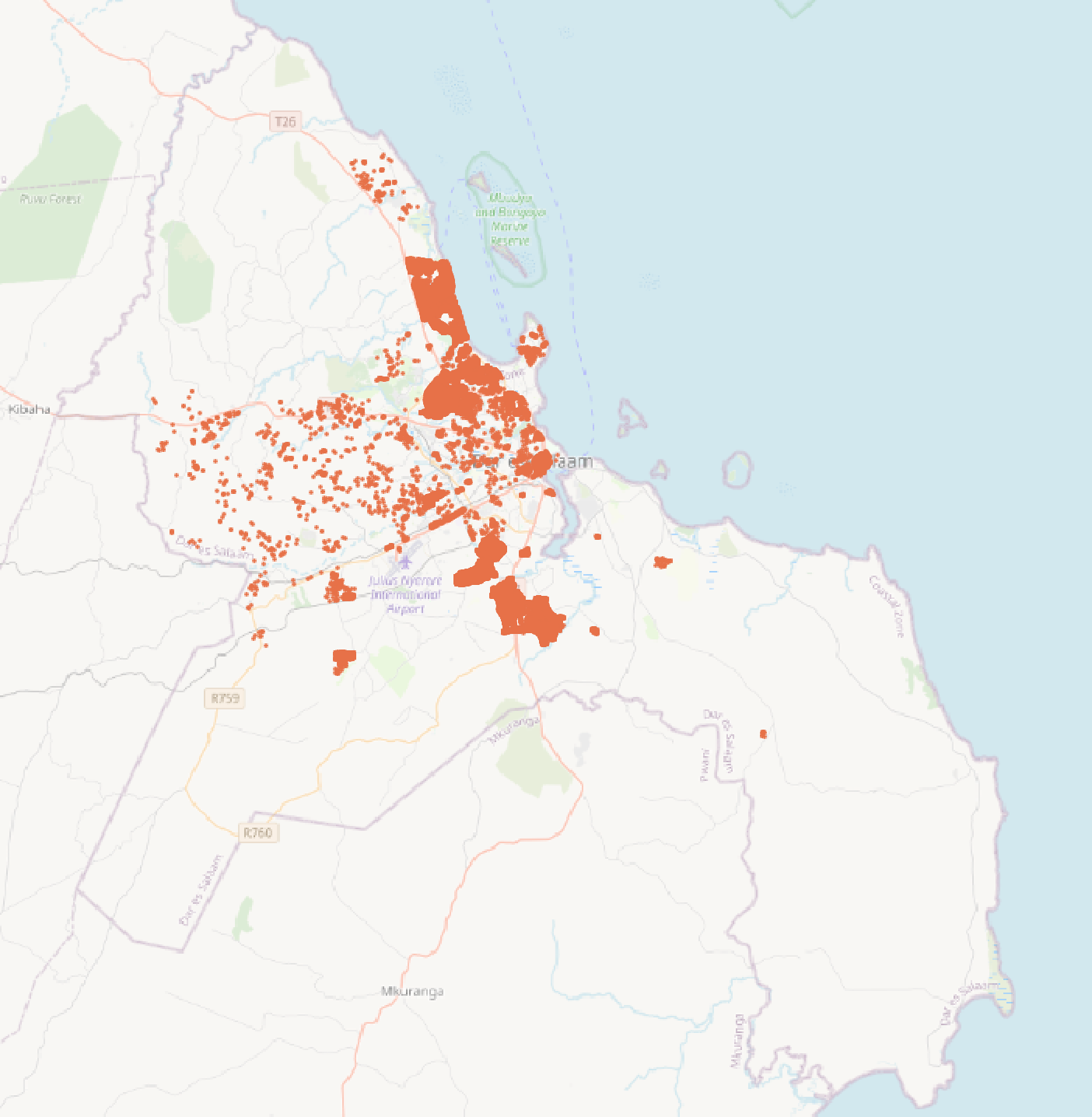
Doing a little bit of math, 11237/12821 = 0.876 and 1311554/1358669 = 0.965, indicating that nonresidential buildings actually make up a greater proportion of the buildings in poor condition than they do buildings in general. This might be partially attributable to more thorough data collection for nonresidential buildings, which could make nonresidential buildings over-represented across all sub-attributes (like building condition, material, and age) that are taken down for some buildings and not others. Also, buildings of a specified good or poor condition are tightly spatially clustered, likely reflecting much more thorough data-gathering in certain parts of the city. OpenStreetMap data for the “building:condition” tag is generally available only where dedicated OSM contributors have spent the most time tagging features.
Spatial Clustering of Buildings in a Specified (Good or Poor) Condition
One last step before analyzing flood risk is to repeat the steps we carried out for buildings in poor condition, but for buildings in good condition, creating a file goodb.geojson and classifying its features into residential/nonresidential. Doing so will allow us to more explicitly examine whether there is a difference in flood risk for a) residential vs. nonresidential buildings and b) buildings in poor condition vs. good condition. The repeated steps are included in the SQL code, but left out here since they are identical to the steps above for poorb.
Among buildings in good condition, we get the following counts, which show that 87.2% of buildings in good condition are residential – probably not significantly different from the 87.6% of buildings in poor condition. Therefore, it seems that neither residential nor nonresidential buildings are more likely to be in better or worse condition. However, they could still experience different levels of exposure to flood risk.
Buildings in Good Condition
| res_status | count_res |
|---|---|
| residential | 60532 |
| nonresidential | 8870 |
Before intersecting buildings with flood risk areas, we can make the process more efficient by dissolving the flood risk geometries into one:
CREATE TABLE flooddissolve
AS
SELECT st_union(geom)::geometry(multipolygon,32737) as geom
FROM flood;
In the very beginning of the workflow, when we downloaded poor/good buildings from OpenStreetMap, we reduced their polygon geometries to single points/centroids with the third line of code (out center;), which will also make the intersection with flood risk areas simpler.
Before carrying out the intersection, we need the building points to be in the same projection as the flood areas geometry:
-- Reproject the poor-condition buildings to EPSG:32737.
CREATE TABLE poorb_reproj
AS
SELECT poorb.*, st_transform(poorb.geom, 32737)::geometry(point,32737) as utm_geom
from poorb;

-- Drop the WGS 84 geometry
ALTER TABLE poorb_reproj
DROP COLUMN geom;

-- Repeat for the good-condition buildings.
CREATE TABLE goodb_reproj
AS
SELECT goodb.*, st_transform(goodb.geom, 32737)::geometry(point,32737) as utm_geom
from goodb;
ALTER TABLE goodb_reproj
DROP COLUMN geom;
Now we can carry out the intersection with an st_within query:
-- Create a boolean field to fill in with risk/nonrisk for each poor-condition building.
ALTER TABLE poorb_reproj
ADD COLUMN atrisk boolean;
-- Set risk to true when the building center-point falls within a flood area.
UPDATE poorb_reproj
SET atrisk = TRUE
FROM flooddissolve
WHERE st_within(poorb_reproj.utm_geom, flooddissolve.geom);
-- Set risk to false when it's not true.
UPDATE poorb_reproj
SET atrisk = FALSE
WHERE atrisk IS NULL;
Poor-Condition Buildings
| atrisk | count_risk |
|---|---|
| False | 11803 |
| True | 1018 |
The same st_within queries can be repeated for the good-condition buildings:
ALTER TABLE goodb_reproj
ADD COLUMN atrisk boolean;
UPDATE goodb_reproj
SET atrisk = TRUE
FROM flooddissolve
WHERE st_within(goodb_reproj.utm_geom, flooddissolve.geom);
UPDATE goodb_reproj
SET atrisk = FALSE
WHERE atrisk IS NULL;
Good-Condition Buildings
| atrisk | count_risk |
|---|---|
| False | 61631 |
| True | 7771 |
Overall, 7.9% of poor-condition buildings are at risk, as opposed to 11.2% of good-condition buildings. Perhaps properties near the water are more valuable, leading to better upkeep of buildings that fall within flood zones. Alternatively, the 3.3% difference might not be very significant, or other factors could be at play. Maybe property owners in areas susceptible to flooding keep their buildings in better-than-average condition in order to withstand potential damage.
Next, we need to calculate the percentages of residential and nonresidential buildings at risk (for buildings in good and poor condition), grouping by wards. With some wrangling, we can also calculate the percentage of all buildings at risk by ward (including those without a specified condition).
First, let’s tidy up our wards data, and join in some population statistics:
-- Edit provided wards data and join census data by ward name.
CREATE TABLE ward_census AS
SELECT wards.*, total_both as totalpop, total_male as male, total_fema as female
FROM wards LEFT JOIN census
ON wards.ward_name = census.ward_name AND wards.district_n = census.dis_name;
-- Transform geometries to EPSG:32737, then drop old geometry.
SELECT addgeometrycolumn('vincent','ward_census','utmgeom',32737,'MULTIPOLYGON',2);

UPDATE ward_census
SET utmgeom = ST_Transform(geom, 32737);
ALTER TABLE ward_census
DROP COLUMN geom;
-- Calculate the area of wards, in case population density is of interest later.
ALTER TABLE ward_census
ADD COLUMN area_km2 real;
UPDATE ward_census
SET area_km2 = st_area(utmgeom)/1000000
FROM ward_census;
The next few steps of code calculate – at a ward level – the percent flood risk of residential buildings in poor condition, residential buildings in good condition, nonresidential buildings in poor condition, and nonresidential buildings in good condition. From this, we can begin to see whether certain kinds of buildings are more likely to be at risk, and whether there are specific wards with high risk for all kinds of buildings. See comments in the code block for details on what the code does.
-- Join ward-level data to the poor-condition buildings, dropping geometries for the time being
CREATE TABLE poor_w AS
SELECT
	poorb_reproj.res_status,
	poorb_reproj.atrisk,
	ward_census.ward_name,
	ward_census.totalpop,
	ward_census.area_km2
FROM poorb_reproj
JOIN ward_census
ON st_within(poorb_reproj.utm_geom, ward_census.utmgeom);

-- Join ward-level data to the good-condition buildings, dropping geometries for the time being
CREATE TABLE good_w AS
SELECT
	goodb_reproj.res_status,
	goodb_reproj.atrisk,
	ward_census.ward_name,
	ward_census.totalpop,
	ward_census.area_km2
FROM goodb_reproj
JOIN ward_census
ON st_within(goodb_reproj.utm_geom, ward_census.utmgeom);

-- Make a new integer field with 1's for risk and 0's for nonrisk so that we can take a sum as well as count
ALTER TABLE poor_w
ADD COLUMN risk int;
UPDATE poor_w
SET risk = 1
where "atrisk" = TRUE;
UPDATE poor_w
SET risk = 0
where "risk" IS NULL;
-- Same, for buildings in good condition
ALTER TABLE good_w
ADD COLUMN risk int;
UPDATE good_w
SET risk = 1
where "atrisk" = TRUE;
UPDATE good_w
SET risk = 0
where "risk" IS NULL;

-- Make a table for poor-condition buildings by ward and (non)residential status,
-- with the number of buildings at flooding risk (sumrisk) and the total number of buildings (count)
CREATE TABLE p_group as
SELECT ward_name,
	res_status,
	sum(risk) as sumrisk,
	count(risk) as count
FROM poor_w
GROUP BY ward_name, res_status;
-- Do the same for good-condition buildings grouped by ward and (non)residential status
CREATE TABLE g_group as
SELECT ward_name,
	res_status,
	sum(risk) as sumrisk,
	count(risk) as count
FROM good_w
GROUP BY ward_name, res_status;

-- Calculate the percent of buildings at risk of flooding, by ward and by residential/nonresidential,
-- for buildings in poor and good condition.
ALTER TABLE p_group
ADD COLUMN pctrisk float;
ALTER TABLE g_group
ADD COLUMN pctrisk float;
UPDATE p_group
SET pctrisk = (sumrisk * 100.0) / (count);
UPDATE g_group
SET pctrisk = (sumrisk * 100.0) / (count);
Next, we can break the percent risk data down into four simplified tables, which we will subsequently join back to the ward_census layer. To do this, we run four queries like this one:
CREATE TABLE p_res AS
SELECT ward_name,
	pctrisk
from p_group
where "res_status"='residential';
The final step is to iteratively join the flood risk data (for each of the four building types) back to the ward_census layer, which still has its original geometries. There might be an easier way to join all four at once, but I simply joined them one at a time:
-- Join back to ward_census (x4, iterative).
CREATE TABLE j1 as
SELECT ward_census.*, pctrisk as poor_res
FROM ward_census LEFT JOIN p_res
ON ward_census.ward_name = p_res.ward_name;

CREATE TABLE j2 as
SELECT j1.*, pctrisk as poor_nonres
FROM j1 LEFT JOIN p_nonres
ON j1.ward_name = p_nonres.ward_name;

CREATE TABLE j3 as
SELECT j2.*, pctrisk as good_res
FROM j2 LEFT JOIN g_res
ON j2.ward_name = g_res.ward_name;

CREATE TABLE j4 as
SELECT j3.*, pctrisk as good_nonres
FROM j3 LEFT JOIN g_nonres
ON j3.ward_name = g_nonres.ward_name;

-- This table (j4) now contains all of the percent risk data for poor/good by res/nonres at a ward level.
-- All that's left to do now is to look into the full set of buildings, including the many that do not have a
-- marked condition.
Results
What we end up discovering is that flooding risk is concentrated in just a few wards, regardless of the type of buildings we are looking at. For instance, the Mikocheni ward has the highest risk for residential buildings in poor condition (91.3% lie in flood zones), and for nonresidential buildings in good condition (64.0% at risk), and falls within the top four wards for risk to the other types of buildings. Generally speaking, the results seem to reflect the proportion of a ward’s area that is covered by flood zones; a more rigorous analysis might examine whether the buildings are spatially clustered within the flood-prone parts of wards, to see whether there are deviations from what we can predict with the proportion alone.
This research into building risk by condition and residential status is limited by the spatial concentration of OSM buildings with a specified condition (good or poor). These buildings appear to have received more thorough data collection than others, and most of them are in central Dar es Salaam. The results of this analysis are representative only of buildings coded with a “building:condition” attribute, so results outside of the city center should be taken with a grain of salt. There are probably significant Type II errors, where buildings at risk of flooding are omitted because they lack a condition attribute. Even so, we can draw interesting conclusions for the areas where many buildings are coded with building condition information. For instance, due in part to the locations of the Msimbazi and Kizinga Rivers, central Dar es Salaam faces considerable flood risk. Furthermore, the percent of buildings at risk varies by ward and by building type, although a handful of wards have high risk across all categories. Some wards have particularly high risk for one kind of building, but not for others – for instance, in Ndugumbi ward the poor-residential buildings are at 41% risk, but good-residential buildings are at only 12% risk. Such differences point to interesting patterns in which certain types of buildings are especially vulnerable to flooding.