Rosgen Stream Classification
Replication authors: Vincent Falardeau, Zach Hilgendorf, Joesph Holler, Peter Kedron, and fellow students in GEOG 0323.
Replication materials available at: https://github.com/vinfalardeau/RE-rosgen
Created: 24 March 2021
Last Revised: 22 May 2021
Introduction
Rivers and streams are defined by dynamic physical processes, dependent on many variables. As such, it is useful to classify streams into types and subtypes that bear similar characteristics, making it possible to discuss streams with a common parlance. Having a classification scheme for streams is important not just for scientists and geomorphologists, but also for planners, watershed managers, and environmentalists, among others. One common scheme is the Rosgen classification, which is used widely, including by the EPA. For the classification to be useful, it should be reproducible – different people should be able to reach the same conclusions about a particular river. In this lab, we aim to reproduce the Rosgen classification carried out by Kasprak et al. (2016) in the Middle Fork John Day Basin, in Oregon. Our reproduction draws on their Columbia Habitat Monitoring Program (CHaMP) data, as well as independently obtained 1-m resolution LiDAR imagery for the study region. By digitizing specific reaches of rivers and their valleys, and using LiDAR to take longitudinal and cross-sectional profiles, we can investigate whether different methods lead to identification of the same stream types.
Methods
Kasprak et al. used a combination of field data, aerial imagery, and 10-meter and 0.1-meter DEMs to infer the broader, Level I valley and stream types of their 33 study sites. In this reproduction, we only used a 1-meter LiDAR DEM and the CHaMP field data, and I investigated a single site. Also, Kasprak et al. used the River Bathymetry Toolkit to derive data about the stream reaches, while we applied a workflow in GRASS GIS and RStudio. In the final analysis, our workflow classified my study site differently than the methods used by Kasprak et al., primarily because the different methods arrived at significantly different entrenchment ratios, and the entrenchment ratio is the very first step in narrowing down the Rosgen classification.
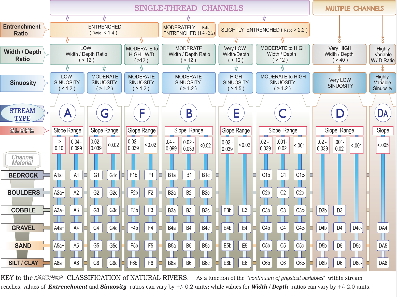
Rosgen Classification Table
Results and Discussion
A number of issues arise when we apply our derived statistics to classifying the stream reach in question. First of all, a cross-sectional transect of the channel and the surrounding valley reveal that the flood-prone area is about 80 meters in width (Figure 3). When we divide that width by the bankfull width, we obtain an entrenchment ratio of 6.47, which is relatively high within the range of values in the Rosgen classification schematic. The high entrenchment ratio indicates that the selected stream reach is hardly entrenched at all, running through a well-worked floodplain that is flat and wide. At this particular cross-section, there is not much downward incision. This leads us to the conclusion that the stream is either Type E or Type C, and we can settle on C due to the high width/depth ratio and low sinuosity. The stream is mostly straight, shallow, and wide. Kasprak et al. came to the conclusion that this stream was of Level I Type B, which includes streams of similar width/depth and sinuosity to Type C, but with lower entrenchment ratios (more entrenchment). This indicates a direction for further investigation, potentially by examining the cross-sections of multiple transects of the stream reach, rather than just one transect – the entrenchment ratio might be variable at different points. A closer look at how entrenchment ratios are calculated in the field might also help to highlight how we obtained a much higher ratio when working with LiDAR data.
The Level II Rosgen classification appears to be more straightforward, as it depends on the slope and the dominant channel material (defined by the median material width). Calculating the rise-over-run for the digitized & derived stream centerline, we get a slope of 0.85%, or 0.0085. From the CHaMP data, we know that the median channel material diameter is 74 mm, which falls within the “Cobble” category for the purposes of the Rosgen classification. Thus, the stream’s Level II subtype is C3 according to our results. Kaprak et al. classify this stream location as B3c, which is also logically consistent with most of our data (width/depth, slope, and channel material) but deviates in the entrenchment, as noted above. Another interesting anomaly is the low sinuosity value we obtained for the stream (Table 2). According to the Rosgen classification table, we should only expect to see sinuosities of less than 1.2 in entrenched, straight Type A streams or in wide, shallow Type D streams. Visually, however, the stream does have some sinuosity in topographic imagery.
Maps, Figures, and Tables
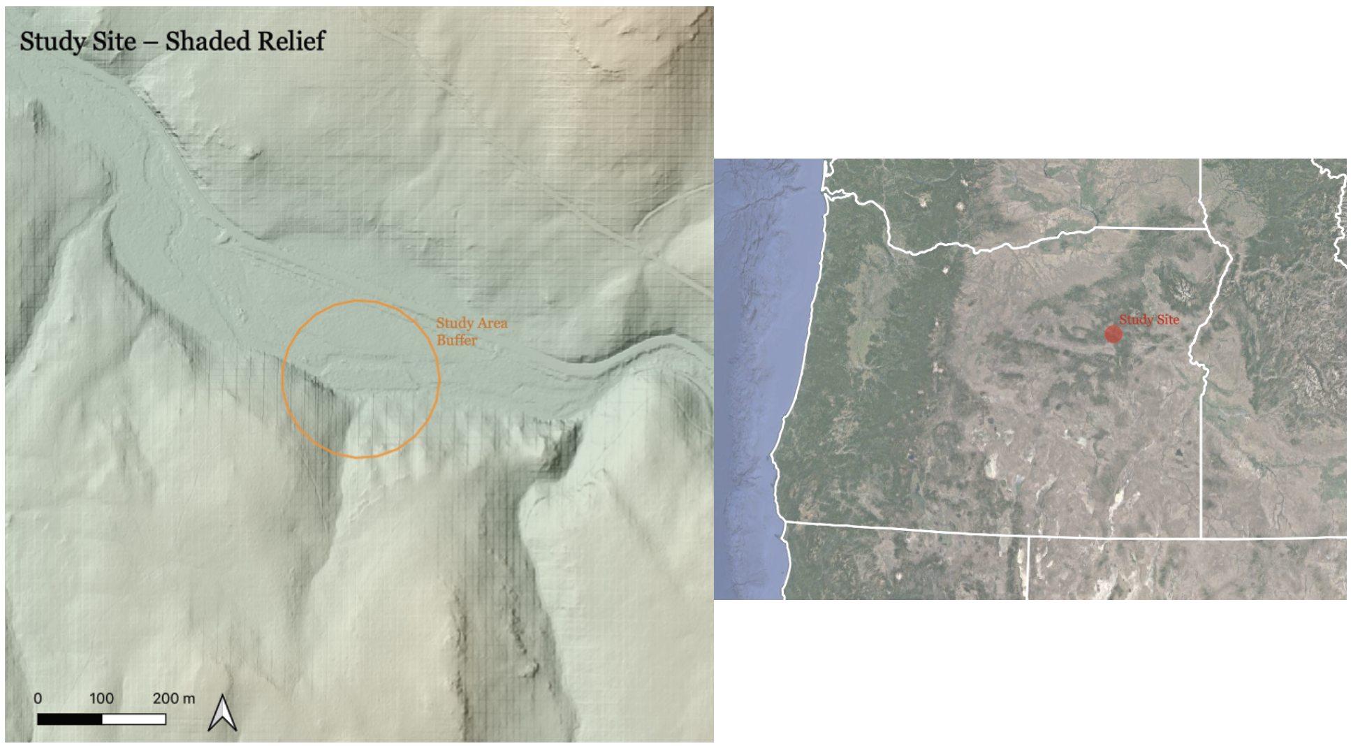
Map 1. A shaded relief map showing the location of the reproduction study site in the Middle Fork of the John Day River in eastern Oregon.
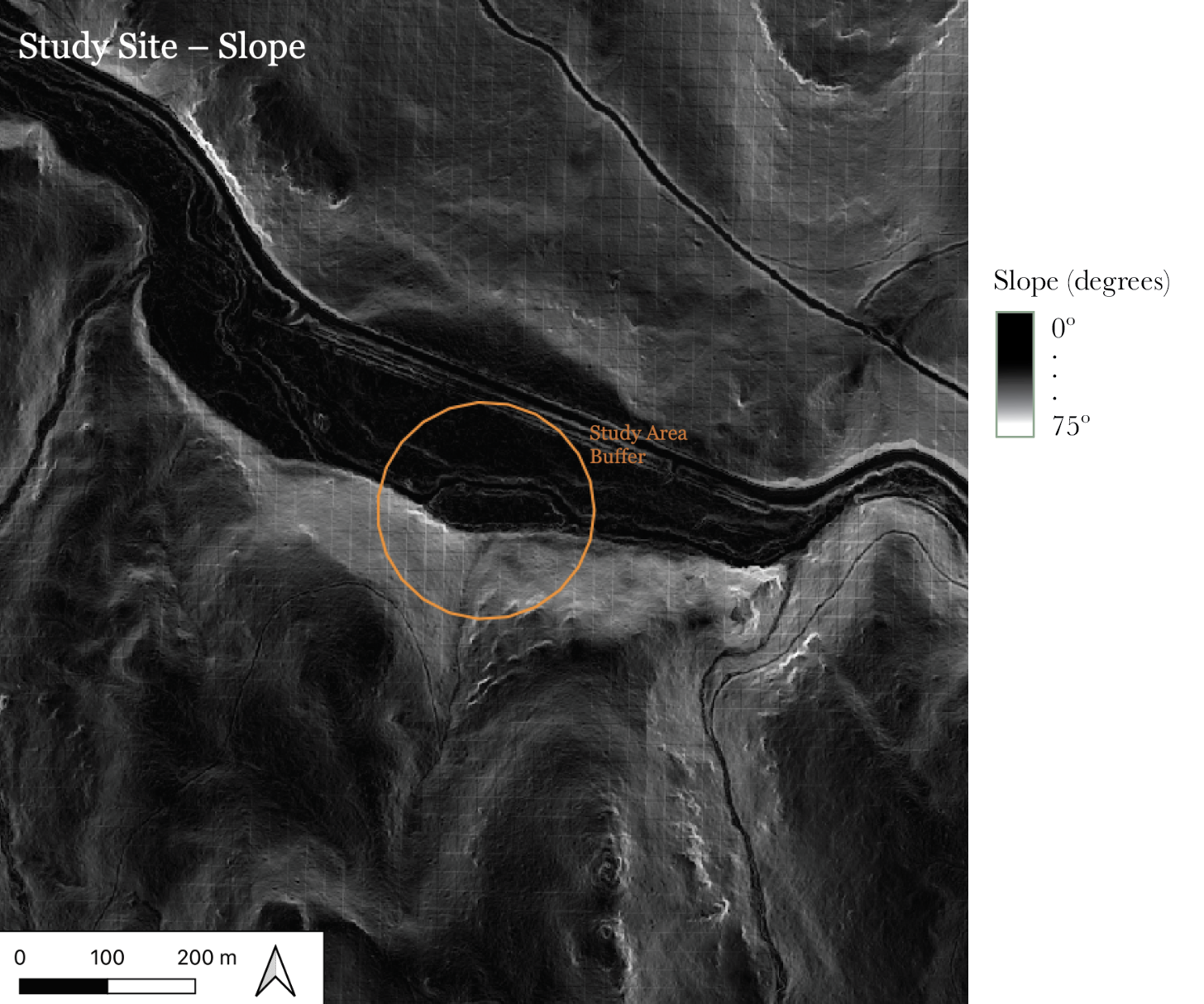
Map 2. The elevation slope, in degrees (the default units in GRASS GIS), around the study location. The floodplain is relatively wide and flat until it reaches steeper slopes in the south and north.
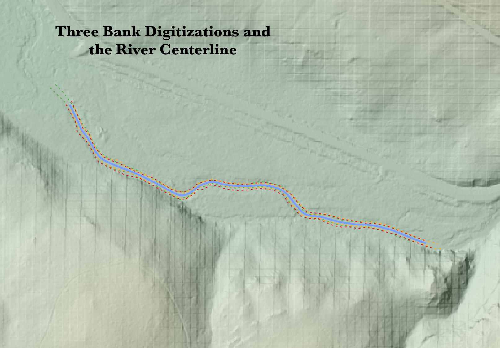
Map 3. Three manual digitizations (dashed lines) of the river’s banks, and a centerline (blue) derived from the six bank lines.
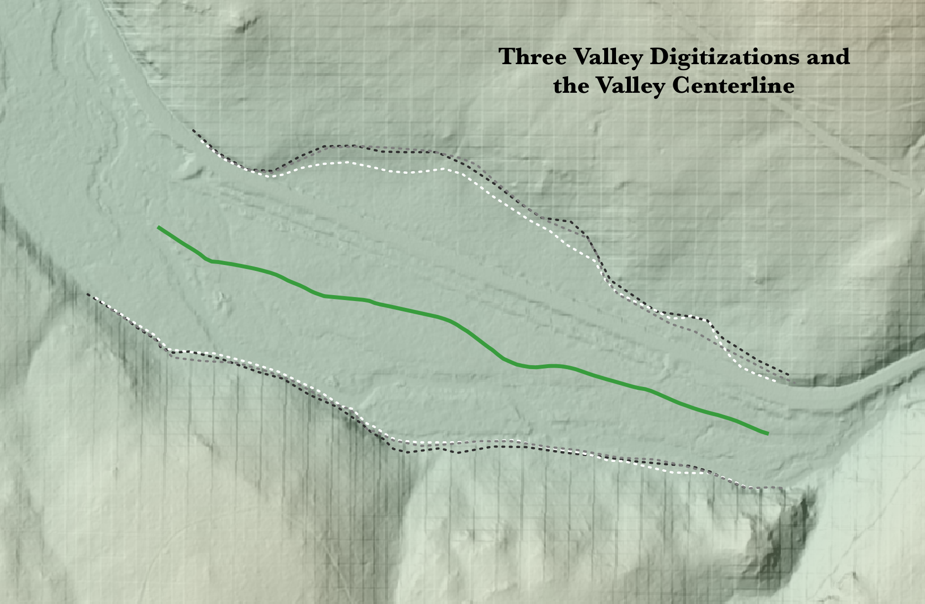
Map 4. Three manual digitizations of the river valley, and a derived centerline (green).
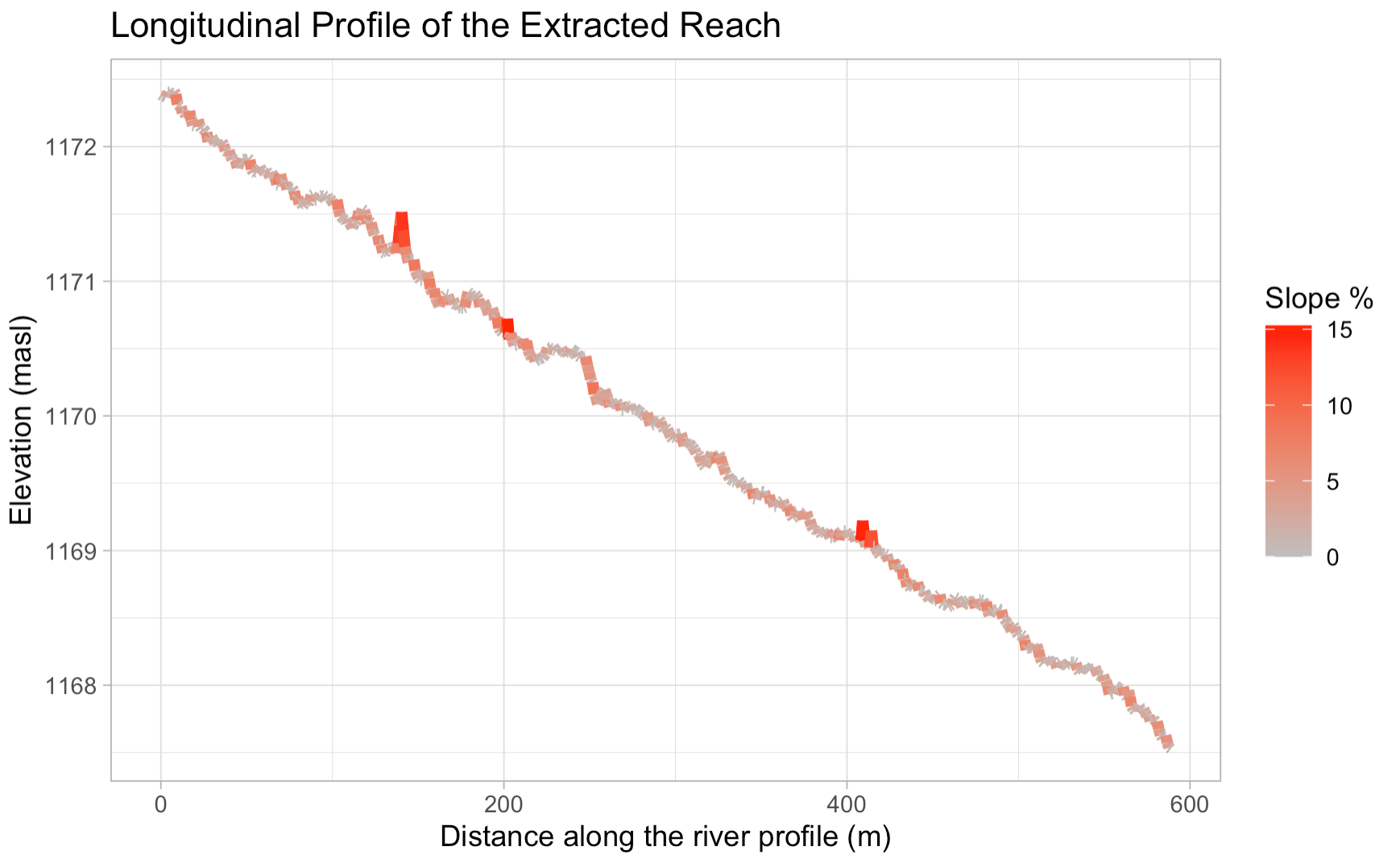
Figure 1. Longitudinal profile of the stream, showing local slope magnitudes (gray to red) and the overall change in elevation of about 5m over nearly 600m, for a slope of 0.85%.
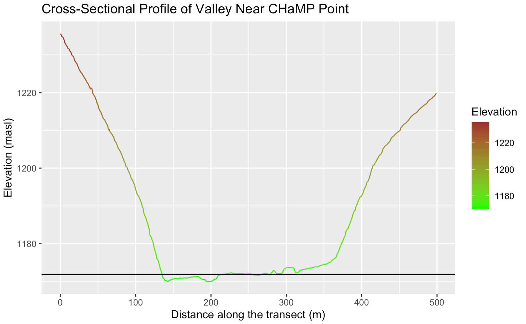
Figure 2. Cross-section of the valley, showing the wide (~200m), flat floodplain between steeper slopes on either side.
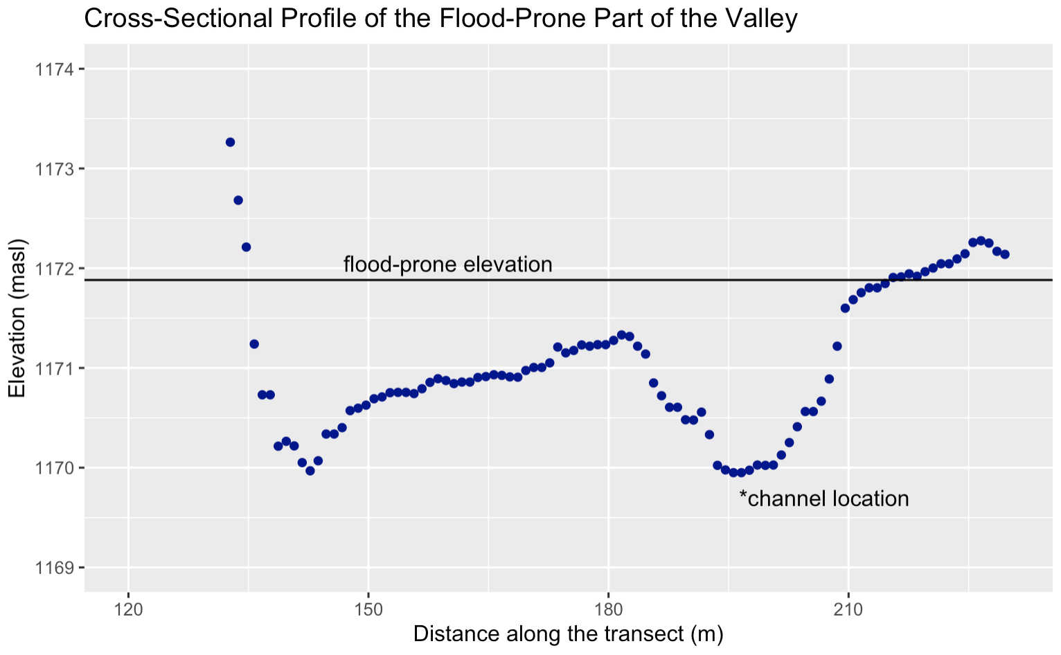
Figure 3. Cross-section narrowing in on the flood-prone part of the valley. Since the stream is not entrenched much, the flood-prone width at twicethe maximum bankfull depth is relatively wide (80m).
Table 1. Site Measurements
| Variable | Value | Source |
|---|---|---|
| Bankfull Width | 12.36 m. | CHaMP |
| Average Bankfull Depth | 0.387 m. | CHaMP |
| Maximum Bankfull Depth | 0.966 m. | CHaMP |
| Flood-Prone Width | 80 m. | LiDAR, CHaMP |
| Valley Width | 190 m. | LiDAR |
| Valley Depth | 3.5 m. | LiDAR |
| Stream/River Length | 632 m. | LiDAR |
| Valley Length | 583 m. | LiDAR |
| Median Channel Material Particle Diameter | 74 mm. | CHaMP |
Table 2. Rosgen Level I Classification
| Criteria | Value |
|---|---|
| Entrenchment Ratio | 6.47 |
| Width / Depth Ratio | 31.03 |
| Sinuosity | 1.08 |
| Level I Stream Type | Type C |
Table 3. Rosgen Level II Classification
| Criteria | Value |
|---|---|
| Slope | 0.85 % |
| Channel Material | Cobble |
| Level II Stream Type | Type C3 |
Conclusion
In this reproduction attempt, I have used high-resolution LiDAR elevation data and locally collected CHaMP data to carry out a Rosgen stream classification at one of the study sites chosen by Kasprak et al. While a sample size of just one location is not enough to make general conclusions about the reproducibility of Kasprak et al, it does not bode too well that this reproduction attempt arrived at a different stream classification of our study site. The main point of disagreement between this reproduction and the original study is on the entrenchment of the stream reach; LiDAR data indicate that the stream is not very entrenched at all, but Kasprak et al find the stream to be moderately entrenched, leading to their Type B classification. With accurate digitization, the sinuosity and slope of a stream appear to be easily reproducible via remote classification from LiDAR data. Entrenchment is more tricky to measure for a number of reasons; for instance, it is variable at a local level, and it is partially dependent on the angular accuracy of the perpendicular cross-section line (any error in the angle would lead to a wider bankfull width). One way to potentially improve the reproduction would be to calculate the entrenchment at regular intervals along the digitized stream reach and compute an average, which might be more comparable to the results obtained in the field. In any case, the reproduction did mostly agree with the original study, since Type C3 and B3c streams are relatively similar. If a process for remote stream classification with LiDAR alone can be developed, it will greatly ease future studies by reducing the burden of research on location.
References
Kasprak, A., N. Hough-Snee, T. Beechie, N. Bouwes, G. Brierley, R. Camp, K. Fryirs, H. Imaki, M. Jensen, G. O’Brien, D. Rosgen, and J. Wheaton. 2016. The blurred line between form and process: A comparison of stream channel classification frameworks ed. J. A. Jones. PLOS ONE 11 (3):e0150293. https://dx.plos.org/10.1371/journal.pone.0150293.
Rosgen, D. L. 1994. A classification of natural rivers. CATENA 22 (3):169–199. https://linkinghub.elsevier.com/retrieve/pii/0341816294900019.